Hand Valve Position Overview Application

 Thumbnail
Mathieu Westerweele
Mathieu Westerweele
Posted on:
2 Sep 2017
A bit more than one year back the company OTS BV came up with an innovative solution to involve Field Operators in Operator Training programs.
A bit more than one year back the company OTS BV came up with an innovative solution to involve Field Operators in Operator Training programs. If you haven’t read about this before or to refresh your memory, please read our previous blog post, or our white paper on this subject and also have a look at a short (2 min) movie clip in which this feature is explained. After discussions with several interested companies a new, very interesting “spin-off” idea grew, which turns out to be very valuable for many companies that have a lot of hand valves (and/or hand operations) in the field. Ideally, in terms of safety and good operation, every valve in a plant or tank terminal should have a position indication that is available in the Control Room. Due to obvious decisions and a balance between risk and costs it is, however, common practice that only very few hand valves have an actual position notifier. The costs when making operation mistakes, due to wrong valve positions (resulting in contamination, spills, production loss, etc.) can be very high. Our “Smart Tag Technology” turned out to be a highly effective and low cost(!) solution to minimize operational risks, by having an overview of the actual valve positions of all (important) hand valves. Since our Smart Tag Technology has already been implemented and used for Operator Training Scenarios (and connected to DCS systems of major vendors), the system can readily be ported to the new functionality. In short: A field operator “scans” the position of a hand valve in the field and, without any delay, the position of this valve is visible on either the DCS or our “Dynamic P&ID Overview” computer system. How it works ATEX NFC Tags are mounted near hand valves.
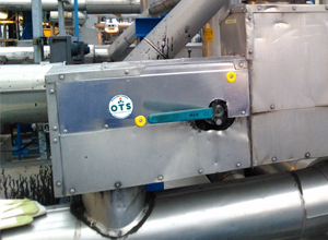
Atex tags
Different embodiments of ATEX NFC Tags
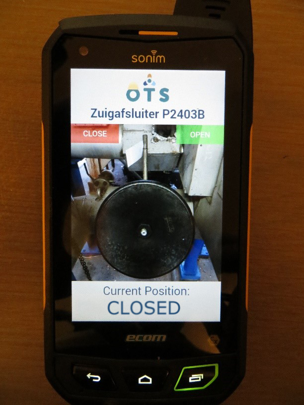
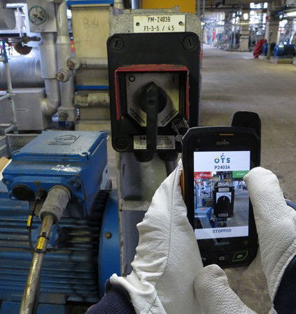
A Tag can be scanned by an ATEX Device (which has the OTS Field App installed), after which the corresponding valve status automatically becomes visible in the control room. The communication between the ATEX device in the field and the software in the control room is done via a (very) secure and dedicated connection.
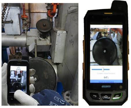
Atex Device
ATEX Device for scanning the Tags
Passing a valve position can be done in several ways. Obviously, it’s up to the end-user to choose which way(s) fits best with their business. Some options we’ve come up with so far, are:
  • After scanning a Tag, an “Open” and “Close” button appear with either a photo of the newly scanned valve, or an icon.
  • A slider appears so that the (approximate) position (between 0 – 100%) can be communicated.
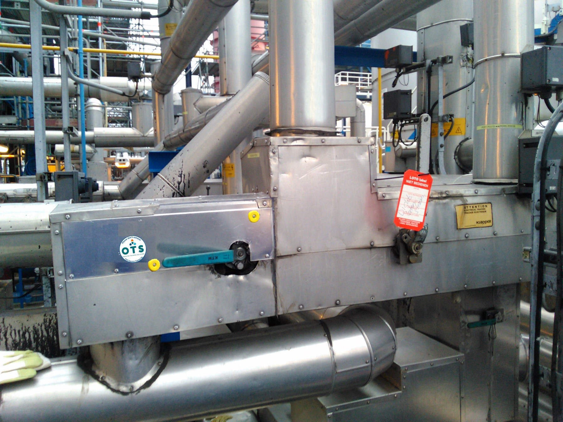
  • There are two Tags mounted near the valve (e.g. a green for Open and a Red for Close), so the operator does not need to do any additional work on the ATEX Device.
  • An overview of several valves appears. By clicking on one of the valves, the position of this valve can be communicated.
  • More options are possible and conceivable.
Hand Valve Tags
Hand Valve with 2 TAGs. One for the “confirmed open” position and one for “confirmed closed”
Atex Device Block Valve
Some more examples of possible interfaces on the ATEX Device.
It’s also possible to pass a desired valve position or a list of desired valve positions (e.g. initiated from the control room) to the ATEX Device. So, after scanning an NFC Tag the actual valve position can be compared to the desired valve position and appropriate action can be taken. The control room has a dynamic overview showing the current valve positions. There are several possibilities for the visualization of the valve positions. Below is an example of a tank terminal, in which the open valves are colored green. The lines in which these open valves are located have a thicker line-weight to indicate that flow is possible. The closed valves in this example are white and the lines are thin.
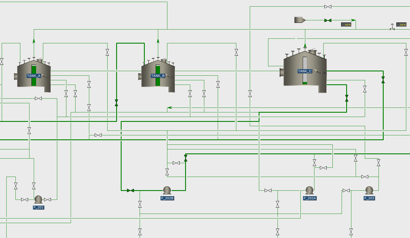
Possible Interface
Some more examples of possible interfaces on the ATEX Device.
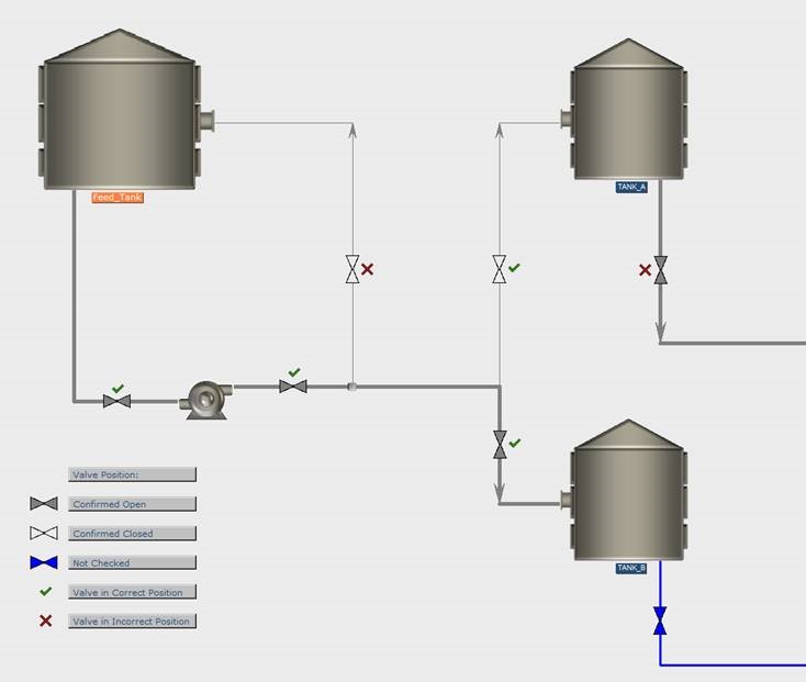
Typically, the P&ID’s are used for the dynamic valve position overviews, but optionally also the DCS screens can be adapted (and connected to the valve position software) to show the valve positions of important valves (and/or to pass desired valve positions to the ATEX Device). In our dynamic valve position overview software you can intuitively browse through all the relevant P&ID’s. Also, the Valve Identifiers (e.g. the P&ID Tag names) can be easily shown or hidden in the overviews. For each valve, a history list is available when it has been scanned and what the position was at that time. If the Field App is being used for trainings, or for certain pre-defined line-ups, which involve a list of valves that need to be checked, the dynamic overview software can display whether a valve has been scanned yet and whether the valve is in the correct position (v) or not (x). When the Tags are in place, they can be used for multiple purposes:
  • Hand Valve Position Overview for all kinds of purposes during normal operation
  • Field Operator training for lining up certain routes.
  • Operator crew trainings. So, control room operators together with field operators, training all kind of scenarios with an Operator Training Simulator.
Dynamic Overview of Training
Example of a dynamic overview for a training.
Are you looking for a robust and affordable solution for monitoring the hand valve positions in your plant or tank terminal? Are you looking for an effective way to train Control Room Operators and Field Operators of your plant? Please contact us fieldapp@mobatec.nl or fieldapp@ots.expert or leave a comment in the comment box below ! To your success! Mathieu. ———————————————–

Introducing “Real Reality” in Operator Training: Field Operator also involved in Simulator Training!

 Thumbnail
Mathieu Westerweele
Mathieu Westerweele
Posted on:
29 Apr 2016
Traditionally, only control room operators are trained with an Operator Training Simulator. However, the real plant is operated by control room operators AND field operators: operations in the control room together with operations in the field determine the performance of the plant.
Traditionally, only control room operators are trained with an Operator Training Simulator. However, the real plant is operated by control room operators AND field operators: operations in the control room together with operations in the field determine the performance of the plant. Especially while handling upsets, starting-up the plant or shutting it down a lot of field operations are required. In those cases communication between all operators involved is crucial.
Several OTS vendors are putting great efforts in developing 3D Virtual worlds to mimic the real plant and although this is great for Greenfield plants or for situations where the team that is to be trained is far away from the actual plant, it remains a form of “serious gaming” at best. Why not use the real plant for realistic trainings?
Our company OTS (Operator Training Solutions) developed a tool to make it possible to train control room operators together with field operators. Please click here to read a recent white paper on the subject. While training, the control room operators use an exact copy of the real DCS. Field operators perform the field operations in the field itself, however not on the real equipment, but via an ATEX approved smart device, connected to the OTS. This is so close to reality that our customer Huntsman refers to this as: Real Reality.
Have a look at this short (2 min.) movie of our satisfied customer to get an impression of how it works:
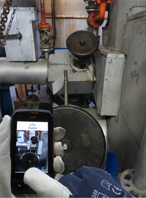
Here are some nice pictures of our Field Operator App “In Action”:
Field Operator
The simulated pump in the OTS can only be operated when the ATEX smart device is close to the real pump in the real plant. The real pump remains unaffected.
Field Operator Field Operator
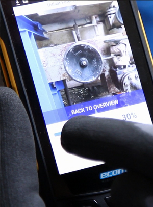
(Simulated) valves can be opened and closed while sliding a ruler to control the speed.
Field Operator
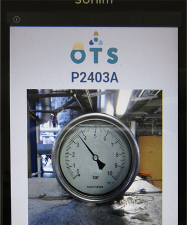
The simulated pressure will be shown on the ATEX smart device only when in the neighborhood of the real pressure gauge.
Let us know what you think about using Real Reality for Training Operator Crews in the comment box below, such that we can all learn something from it.
To your success!
Mathieu.
———————————————–
PS: please browse to our OTS website to learn more about our Operator Training Solutions

Steady-State Assumptions

 Thumbnail
Mathieu Westerweele
Mathieu Westerweele
Posted on:
30 June 2014
Last month we had a look at modelling challenges that can arise when making constraining assumptions. This month’s blog will cover a related form of constraining assumptions, the steady-state assumption.
The need for (pseudo) steady-state assumptions may arise for different reasons. Often the purpose is to either simplify the dynamic behaviour of the system by idealising components or it is to compensate for information that is not readily available or difficult to model for other reasons.
The idealisation of components is context-wise related to the subject of singular perturbation. Since the model is built for a specific purpose, one may choose to ignore the dynamic effects of certain parts of the system and assume that they are either extremely slow thus can be approximated as reservoir providing an infinite-size source of matter, energy, etc., or one may make assumptions of instantaneous dynamics for small-capacity parts.
If you critically analyse models, as they are published in the literature, you will find that such assumptions are omnipresent. In fact they are intrinsically in the basics as models are mostly build on the assumption of reversibility, which does imply that one deals with small capacity elements that move along trajectories on the equilibrium surface.
One often finds problems where two systems of largely different nature are coupled. For example a large system that is connected to a small system. Often the dynamic effects of the small system may be ignored, but very often too, the small system makes all the difference. Models in which a phase transition takes place are of this nature in that the phase boundary separating the two phases is very important when describing the flow of mass from one phase to another. This concept may also be applied to time scales, such as fast and slow systems. For these systems the singular perturbation theory is applicable. For fast systems a pseudo steady-state assumption is made:

ε dx/dt = A z + B r


which yields

0 = A z + B r

if ε := 0.
The capacity effects of the fast systems are omitted and this reduces the state of the process because the dynamic equations of this parts are set to zero. The state of a fast capacity becomes a function of the state of its environment, which mathematically reflects into the elimination of the state. So, for these fast systems the accumulation terms vanish and, consequently, the primary state variables are undefined for these systems. The balance equations of the fast systems are still valid and are used to calculate undefined variables either directly or indirectly. Quite obviously, an “unmodelled flow” can be calculated directly via a steady-state assumption.
In general, a number of steady-state assumptions that remove n states result in the following set of algebraic equations (only for the fast capacities; see the blog post on structurally consistent models for a notion of what these equations and variables represent):

0 = A z + B r


y = f(x)


z = g(y, ye)


r = h(y)

from which n variables (either flow rates (z), reaction rates (r) and/or states (x or y)) can be calculated (less variables can be calculated when index reduction algorithms affect the steady-state balance equations). In this set the ye represent the (secondary) states of the environment systems (i.e. systems that are connected to the steady-state systems) and are the driving forces of the algebraic equations. A bipartite graph analysis could provide the means for finding the different sets of variables that can be computed from this set of algebraic equations. Normally, though, each steady-state assumption can be handled locally and it is clear for which variables the equations are solved.
Consider the following example of a simple heat flow though a thin wall:
Heat Flow
Figure A: simple process; a heat flow through a thin wall.
Figure B: (possible) Physical topology of this simple process
Three systems are interconnected via heat connections. The enthalpy balance of the middle system (2) of figure B is:

d(H)/dt = qa − qb

If the second flow (qb) remains “unmodelled”, then a steady-state assumption (on system 2: d(H)/dt := 0) can be made to calculate this flow via the balance equation:

qa = qb

If there would have been no inlet flow to system 2 and a steady- state assumption is made, this would, of course, result in no flow through connection 2 (i.e. qb = 0).
As mentioned, the steady-state assumption essentially makes the state of a system a function of the state of its environment. The state of the environment can thus be used to redefine the (secondary) state (i.e. the intensive quantities) of the system.
Consider figure B once again. The heat ows through the connections a and b are now defined as functions of the temperatures of the interconnected systems:

qa = U1 A1 (T2 − T1)


qb = U2 A2 (T3 − T2)

If a steady-state assumption is made for system 2, the primary state of the system is eliminated and, consequently, also the secondary state, because this results from a mapping from the primary state. The temperature T2 of system 2 is now defined as a function of the states of the environment (T1 and T3) and can be calculated from the balance equation of this system:

0 = qa − qb
⇔ T2 = (U1 A1 T1 + U2 A2 T3 ) / (U1 A1 + U2 A2 )

Note: When one or both flows remain unmodelled, the balance equation of system 2 is effectively removed from the model by applying the Simple Index Reduction Method. The introduced constraint (e.g.: T2 = T1 and/or T2 = T3) equations are then used to calculate T2.
The two examples showed that a steady-state assumption can be used to either calculate an unmodelled flow (or reaction) directly or calculate the (secondary) state of the system that is redefined by its environment. Both possibilities do not lead to index problems, since the states are removed directly from the model description.
These two possibilities can, however, not be mixed, because one would run into mathematical problems. If, for example, the inlet flow qa is defined as qa = U1 A1 (T2 − T1) and we wish to calculate qb via a steady state assumption, there would be a problem because there is no information on the temperature T2. When the steady-state assumption calculates the state of a system, then at least one of the connections must, of course, reference this state. Otherwise the resulting set of equations will be inconsistent and it will not be possible to calculate the state.
Conceptional diffculties arise when a steady-state assumption reduces a system that is connected with more than two connections that remain “unmodelled” (and for which no constraint equations are given). In these cases, one of the flows is calculated via the steady-state assumption and the other flows are defined as a function of the calculated flow. So, in these cases, some flows can be a function of another flow and not, which is the general case, of the state variables of the connected systems.
What is your experience with steady-state assumptions? Did you ever run into computational problems without knowing what the cause was?
I invite to post your experiences, insights and/or suggestions in the comment box below, such that we can all learn something from it.
To your success!
Mathieu.
———————————————–

Overflowing Tank Example

 Thumbnail
Mathieu Westerweele
Mathieu Westerweele
Posted on:
30 May 2014
We will take a look at an example of an assumption that will lead to a high index model, but first we will look at the same example with no constraining assumptions:
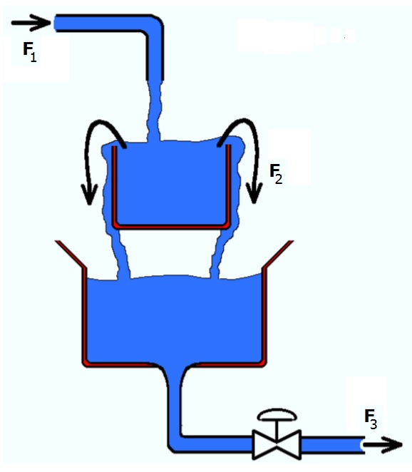
A process consists a mixing tank that flows over into a second tank (see figure). The liquid that is fed to the tank system contains two components (A and B). We are interested in the (dynamic) concentration change of the components (in the first tank) over time.
In a previous blog post we discussed about constraints and assumptions that describe all kinds of algebraic relationships between process quantities which have to hold at any time.
As mentioned, these assumptions are usually introduced with a goal, namely to simplify the description of the behaviour by neglecting what is considered insignificant in the view of the application one has in mind for the model. Whilst indeed such assumptions do simplify the description, they are also the source of numerous problems, such as “index problems”, which make the solving of the equations very difficult.
We will take a look at an example of an assumption that will lead to a high index model, but first we will look at the same example with no constraining assumptions:
A process consists a mixing tank that flows over into a second tank (see figure). The liquid that is fed to the tank system contains two components (A and B). We are interested in the (dynamic) concentration change of the components (in the first tank) over time.
To keep the explanation simple and easy to follow, the (mass and molar) density will be considered to be constant and we will only consider mass. A well posed system of equations could look as follows (you will see a list of equations. In front of each equation is noted which variable is being solved from this equation):
 

Balance equations:

n_A:  d(n_A)/dt = F1_A – F2_A
n_B:  d(n_B)/dt = F1_B – F2_B
 

System equations:

c_A:  c_A * V = n_A
c_B:  c_B * V = n_B
m:    m = M_A * n_A + M_B * n_B
V:     m = Dm * V
 

Connection Equations:

F1_A:  F1_A = c_A0 * F1
F1_B:  F1_B = c_B0 * F1
F2:     IF V > Vmax THEN
           F2 = K * (V – Vmax)
         ELSE
           F2 = 0
         END
F2_A:  F2_A = c_A * F2
F2_B:  F2_B = c_B * F2
Where:
n_i :: molar mass of component i, in [mol]
c_i :: molar concentration of component i, in [mol/m3]
m  :: total mass, in [kg]
M_i :: molar mass of component I, in [kg/mol]
V  :: Volume of system, in [m3]
Dm  :: density in [kg/m3]
F#  :: Volumetric flow rate of connection #, in [m3/s]
F#_i :: molar mass flow of component i through connection #, in [mol/s]
K  :: Constant, in [1/s]
F1 and c_i0 are a function of boundary conditions and can be considered given.
Note: The equations F2 = K * (V – Vmax) is a simplification that seems to work very fine in most situations. It just means that the higher the value of V (above Vmax), the bigger the flow F2 will be. It will automatically find an “equilibrium value”. The K represents a measure for the “resistance to overflow”. If K has a very high value, V will always be close to Vmax.
Let’s now suppose that it was diffcult to find a reliable relation that describes the flow F2 out of the overflow tank. Therefore the assumption is made that the liquid level in the tank is constant (this means that the liquid volume dynamics are assumed to be very rapid compared to the composition dynamics, which is theoretically the same as taking K equal to infinity). So, we now have a constraint that V = Vmax and we no longer have an equation to calculate F2.
This assumption of constant volume is, of course, physically incorrect. A physically more correct description of the overflow would have included a relation between the liquid level and the amount of liquid which is flowing out of the tank (for example the equation for F2 in the well posed model). Though practically, the variation in the volume is hardly ever relevant in these circumstances and the resulting low index model will be stiff.
So, let’s have a look at the equations that would be needed for this simple model and how the simplifying assumption can lead to a “high index model” that is hard to solve for most equation based solvers.
(1) d(n_A)/dt = c_A0 * F1 – c_A * F2
(2) d(n_B)/dt = c_B0 * F1 – c_B * F2
(3) c_A * V = n_A
(4) c_B * V = n_B
(5) m = M_A * n_A + M_B * n_B
(6) m = Dm * V
(7) V = Vmax
The equations for this model are, of course, almost the same as the ones for the previous example. The only exception is that there is no longer an equation to solve F2 from and instead we have a constraint on the total volume. The problem with solving this set of equations is that the variable F2 does not have an equation but does appear in the balance equations, which will be impossible to solve for most equation based solvers (some solvers have built-in index reduction algorithms, but that’s not the topic of this blog).
One way of “transforming” this set of equations into a set that can be solved, is to apply an index reduction by differentiating some of the equations.
The constraint equation (V = Vmax) constrains the volume and makes the volume V no longer state (nor time) dependent. The volume is related to the mass of the system (equation 6) and the mass is related to the component masses (equation 5). Differentiating equations (5) and (6) results in:
(5’) d(m)/dt = M_A * d(n_A)/dt + M_B * d(n_B)/dt
(6’) d(m)/dt = 0
which results in the following additional algebraic equation:
0 = M_A * c_A0 * F1 + M_B * c_B0 * F1 – M_A * c_A * F2 – M_B * c_B * F2
Removing one of the states of the original equations (either n_A or n_B) and replacing its differential equation with the new algebraic relation results in an index-1 DAE, which can be easily solved by a DAE solver.
Quite obviously, when the new algebraic equation is worked out, it will follow that, in this simple case (constant density), the volumetric outflow F2 will be the same as the volumetric inflow F1:
0 = (M_A * c_A0 + M_B * c_B0) * F1 – (M_A * c_A + M_B * c_B) * F2
0 = (M_A * n_A0 + M_B * n_B0) * F1/V0 – (M_A * n_A + M_B * n_B) * F2/V
0 = m0/V0 * F1 – m/V * F2 = Dm*F1 – Dm*F2
==> F1 = F2
Note: Very often, similar examples are used in textbooks without anybody noticing that there is (or was) an index problem related to the example. This has the following reasons: The total mass balance and all but one component mass balances (mostly the solvent is left out) are written down and, without knowing it, no link is being made between the component masses and the total mass:
d(m)/dt = Dm*F1 – Dm*F2
d(n_A)/dt = F1_A – F2_A
c_A = n_A / V
V = m / Dm
Making the assumption of constant density and constant volume results in constant total mass, which easily gives:
0 = Dm*F1 – Dm*F2 ⇒ F2 = F1
When a modeller is not aware of the fact that the component masses were not related to the total mass in this case, he could get into trouble when things get a bit more complicated (for example when the density is a function of the mole fractions). So, while this solution works fine for “academic” problems, it’s not always wise to solve industrial problems this way. Unfortunately, many engineers are often not even aware of the assumptions they are taking and what the implications of such assumptions can be.
What is your experience with constraints and assumptions? Did you ever run into computational problems without knowing what the cause was?
I invite to post your experiences, insights and/or suggestions in the comment box below, such that we can all learn something from it.
To your success!
Mathieu.
———————————————–

How-To Tutorials on YouTube?

 Thumbnail
Mathieu Westerweele
Mathieu Westerweele
Posted on:
30 Apr 2014
I will probably “cross the line” a bit with this month’s blog topic, since it will deviate from the other blogs I have written so far and will not focus on modelling in general. But, I promise I will make it worth it for both of us, if you continue reading until the end ;).
We were brainstorming with our team a few weeks ago about good ways to “bring our message to the world”. As you might recall:
————
It is our goal to bring our modelling methodology to the world and to teach engineers that modelling can be quite easy and very valuable.
Our software tool, Mobatec Modeller, which is developed within our company, builds on this modelling methodology. Process models of any size can be built; from a single unit to entire processing plants (resulting in more than 100.000 equations). There is a wide application range for these models in e.g. research activities, on-line predictions, control and operator training simulators.
Mobatec Modeller is a software package that helps the model builder to setup the (mathematical) model of any process. The tool significantly reduces the time needed to produce a working (!) dynamic or steady-state process model. Models that are developed in Mobatec Modeller are set up in such a way that it is possible for any process engineer to quickly understand the structure of the model and the assumptions made for this model. You don’t have to be “the designer” to understand the model, it is really that easy!
Mobatec Modeller has been set up to be a user-friendly tool to define and modify dynamic process models. Even beginning users can quickly set up complex models that are transparent for others without the need for extensive documentation.
We believe it is possible to take process engineering to a higher level in both industry and academia. Since we have experienced the benefits in using this new approach, we want you to be part of it!
————
That all sounds great, of course. We would, however like more people to know about our solutions.
We are a small group of purely technical oriented people, making our product better and better. We are telling the world about this via our website and by making our software freely available for download (with some restrictions, of course, such as not being able to store your models). We made easy-to-follow Learning Modules, integrated in the software. We make sure we have very satisfied customers (feel free to ask for references 🙂 ).
But are people able to find us online, if they have a question for which a (dynamic) simulation model could offer them a solution?
The latest idea we had, was to record several “How-to Tutorials” and place them on YouTube. The result of our first attempts can be found on www.youtube.com/mobatecmodeller. In my opinion this is a great way to show beginning users to solve basic problems they might have. It’s also a great way to interest people, who don’t know us yet, and to show them what can be done with our powerful tool (although we can, obviously, not show everything).
We are in this business to help you and others to solve (engineering) problems that you might have. We only do business with clients that we know who will benefit from our solutions. This will make both parties happy, in the end. I truly believe in win-win solutions, in business as well as in my personal life. Therefore, I feel it is only fair that we give you value if you give us valuable information (and vice versa, of course).
We have several questions that we would like to have your help with:
How can/should people find us online?
Is such a YouTube channel indeed a good idea?
In which way can we improve our online tutorials?
How do we reach a large audience and let the world know about our powerful modelling tool?
Are there other ways than videos and one-on-one teaching sessions?
In return for positive and helpful reactions to these, and maybe more, questions, we will reward you… 😉
Mobatec Wine
So, please share your ideas or suggestions on how to make the dynamic modelling and simulation tool Mobatec Modeller known to a large audience, such that we can help people around the world to make their (modelling related) problem solving easier.
Feel free to post your experiences, insights and/or suggestions in the comment box below, such that we can all learn something from it.
To your success!
Mathieu.
———————————————–