The modelling methodology behind Mobatec Modeller assumes that any process can be broken down into systems and connections. Systems represent a capacity, able to store mass and energy. Connections represent the transfer of mass and energy between the defined systems.
So far, however, we have dealt with “lumped” systems as a basic modelling element. Lumped systems are assumed to have uniform properties over their entire volume. A typical example of such a system is a simple (one phase) CSTR, as the whole volume is assumed to be ideally mixed. In that case, mathematically speaking we are calculating the assumed “uniform point” properties & behaviour and are using the volume of the system to quantify the system, i.e. calculate the defined system performance. From a mathematics point of view this is DAE (Differential Algebraic Equation) problem, containing Ordinary Differential Equations (ODE) and Algebraic Equations (AE), where the time is only independent variable. ODE’s are representing the balances (mass & heat) equations of the systems while AE’s are called constitutive equations and are used to define each system properties.
What is a modelling strategy towards non-uniform systems?
A cascade of lumped systems can be used to simulate (already existing) non-uniform systems successfully enough, but if the model goal is the design, optimization and model based innovation of such systems, then the model made would need to take spatial coordinates of the modelled system into account as independent variables as well. From mathematics point of view this problem then becomes PDAE – Partial Differential and Algebraic Equations problem. In this months blog we are going to talk about the Distributed Parameter System modelling in Mobatec Modeller, a solution strategy, and numerical methods used.
Distributed parameter systems are systems that cannot be considered to have uniform properties over their entire volume, hence they are called “distributed parameter” as their properties are time and space dependent.
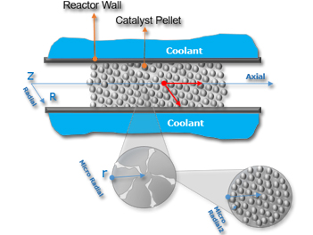
Typical representatives of such a systems are plug flow & packed bed reactors, fixed or moving bed columns, catalytic pellets, etc.
Dominant phenomena in these systems are convective and dispersive/diffusive mass & heat transfer. In order to solve these type of problems space discretization numerical methods are required.
Space discretization numerical methods in Mobatec Modeller
Numerical discretization of a time-dependent partial differential equation (PDE) includes the following approaches: Fully-discretized in both time and space and Method of Lines. In Mobatec Modeller we employ the Method of Lines approach (MOL). (MOL) approach: discretize in space first, transform PDEs to ordinary differential equations (ODEs); and then using the time integration method of ODEs to advance in time.
There are several spatial discretization methods: Finite Difference Method (FDM), Finite Volume Method (FVM), Finite Element Method (FEM), Spectral and Pseudo-spectral Method. Finite Difference Methods (FDM) are adopted as dominant approach to numerical solution of PDE’s and are used in Mobatec Modeller.
Finite Difference Methods make derivatives approximation of univariate functions by replacing the derivatives in equations with finite difference approximations. This results in a number of ordinary differential & algebraic equations that can be solved simultaneously. The basic idea of finite difference schemes is to replace derivatives by finite differences. The most common method of obtaining the finite-difference expressions is via Taylor series expansion: 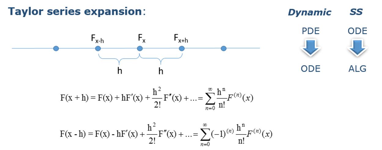The Taylor series expansions for the nearby points of Fx are used to obtain the First and later the Second derivative approximations at Fx. Depending whether we employ expression for the point before F(x-h) or the point after F(x+h) the point Fx, or combine both expressions together we will get: Forward, Backward or Central Finite Difference approximation of the derivatives. (FFDM, BFDM & CFDM)
Forward and Backward finite difference methods can be used alone, depending on the boundary conditions provided for the system, i.e. do we know the inlet or the outlet boundary condition. If we want to employ a central finite difference method then all three methods are needed to form a numerical solution strategy. This will be explained in detail later on, but let us first “get to know” each method separately: 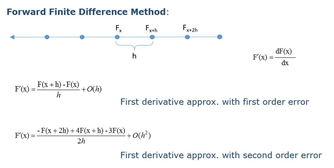FFDM is using the point after the focus point. The arrow tip is showing the integration direction, which is from Z=Z towards Z=0. So we use FFDM if the outlet BC is known. 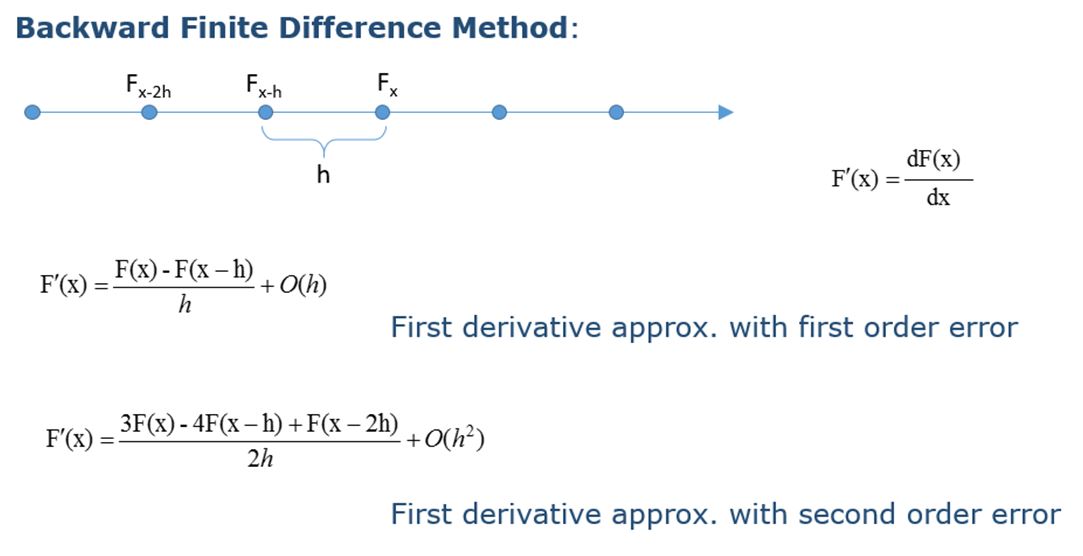BFDM is using the point before the focus point. The arrow tip is showing the integration direction, which is from Z=0 towards Z=Z. So we use BFDM if the inlet BC is known. “O” is representing the terms in the Taylor series expansion that are being neglected and is representing the error of the finite approximation. First order error is of the order of spatial step taken O(h). Second order error derivative approximation is obtained by including one more point in the approximation expression. For FFDM that is F(x+2h) point, and for BFDM is F(x-2h) point. The error is of the order of spatial step squared O(h2) which is more accurate solution taking that h->0. 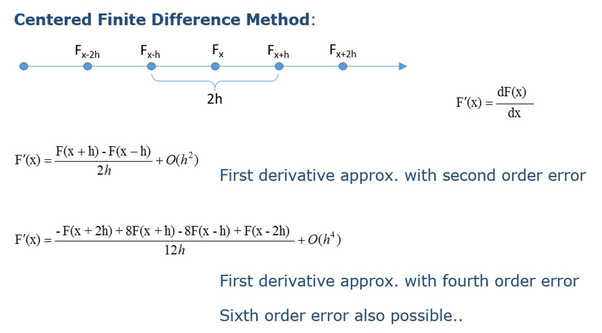CFDM is using the point before and the point after the focus point. The arrow tip is showing the integration direction, which is from Z=0 towards Z=Z. In order to employ CFDM we use BFDM at the inlet BC point and FFDM at the outlet BC point. In the middle – throughout the distributed domain CFDM is used. This subject will be tackled in detail in a next blog once we get to know the methods properties.
Below, the graphical interpretation of the finite difference derivatives approximation by used method is given: 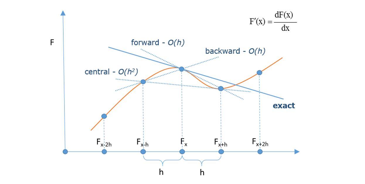The smaller the spatial step (h->0) the better the finite approximations of the derivatives are. The same goes with higher error order. In real case the desired solution would be an optimal number of spatial elements (spatial step size) over the distributed domain length. Too much spatial steps -> very small step size h, would take too much computational time and effort.
Let us take a look at the second order derivatives finite approximations. If we take the derived first derivative finite approximations and reuse them in the Taylor series expansion, now deriving the second derivative finite approximations we will get: 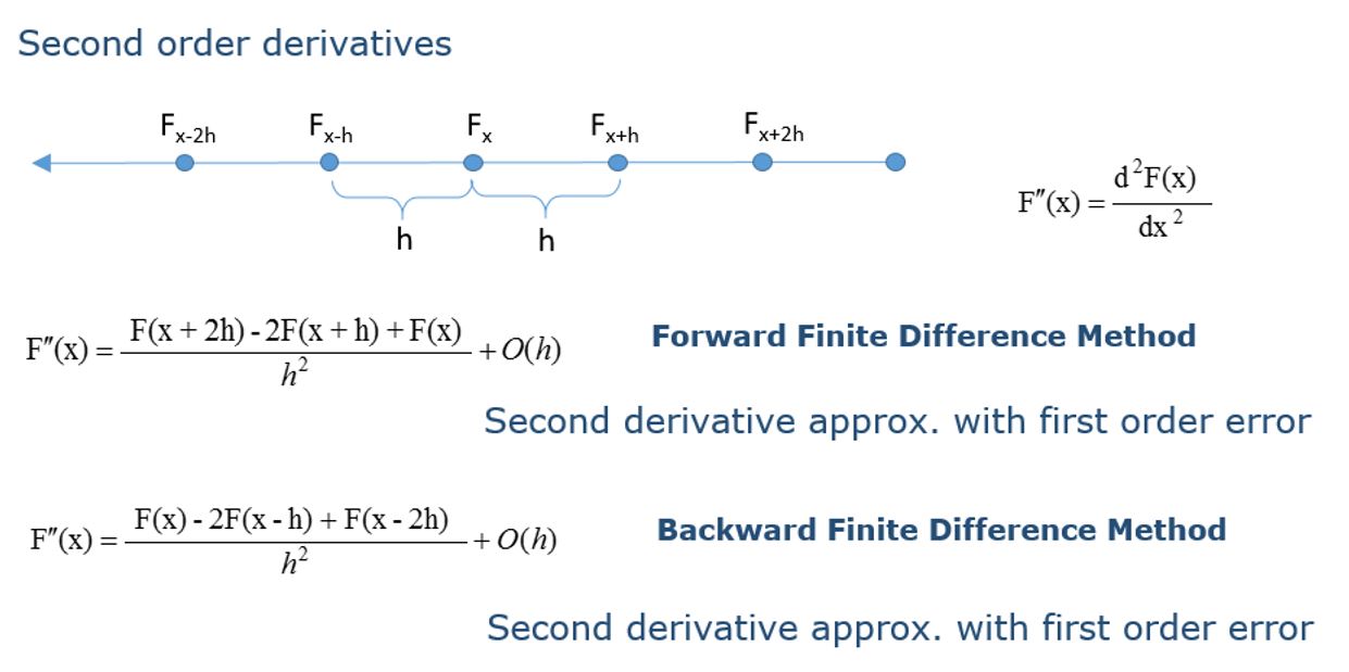The error order is of the spatial step size so they are not used that much. Main use is for purely convective terms -> first derivative finite approximation.
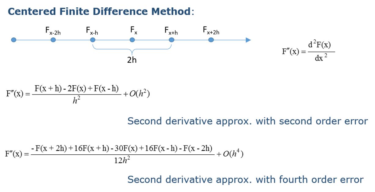CFDM can be successfully used for mixed convective and (purely) diffusive/dispersive terms. Knowledge on numerical methods is essential for their successful application in real life engineering problems. In the next blog on this topic, we will explain the application of FD methods in Mobatec Modeller and why it is important that this part of the PDE solution strategy needs to remain a “white box” – available for user to interact with in order to be able to make the models to converge and not have their hands “tied together”.
What is your experience with Distributed Parameter System modelling and numerical methods used? Did you ever run into convergence problems without knowing what the cause was?
I invite to post your experiences, insights and/or suggestions in the comment box below, such that we can all learn something from it.
To your success! Vladimir.